Data science specialization – Coursera – Word prediction with R
Introduction
Data Science is an interdisciplinary field that deal with methods, processes and systems for extracting knowledge contained in structured or unstructured data. The data mining process usually depends of a series of steps, the image below shows the standard path that a data scientist usually take.
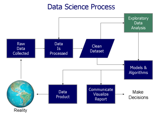
At each step of the Data Science process, several activities are required, eg: choice of models and mining algorithms, communication modes for presentation of results, forms of collection, exploratory analysis, pre-processing, etc.
For this project we used the R programming language and the RStudio development IDE. R is a free software environment used for statistical activities and graphing, it compiles and runs on a variety of UNIX, Windows and MacOS platforms.
Objective
The purpose of this paper is present the data science process with a practical scenario. Content with practical examples to explain the complete flow of the data science process make easy the learning process. Will be demonstrated step by step how to create an application for word suggestion during text writing. This work was applied to obtain the title of specialist in Data Science of John Hopkins University in Coursera. The project is available on GitHub in the repository Data Science Capstone.
Project
Around the world, people spend a lot of time on their mobile devices in a series of activities that require writing, such as sending e-mails, social networking, banking transactions, etc. This project builds an intelligent algorithm to suggest to people the next word of a sentence, for example if someone types:
I go to
The keyboard can suggest three options of what the next possible word would be. For example: gym, market or restaurant. So the following steps will present the complete process to create this application.
1 – Obtaining the data
The dataset used to build this project was provided by the company SwiftKey. The first task is obtain the dataset and understand how it is organized. We first make the data download and extraction with the following code:
# Valid directories and variables
dir_data <- "data"
dir_data_raw <- "data/raw"
dir_data_raw_final <- "data/raw/final"
zip_data_file <- "Coursera-SwiftKey.zip"
zip_data_url <- "https://d396qusza40orc.cloudfront.net/dsscapstone/dataset/Coursera-SwiftKey.zip"

# Obtaining the data from the WEB
if(!dir.exists("data")) {
    dir.create(data_dir)
}
if(!file.exists(sprintf("%s/%s", dir_data, zip_data_file))) {
    download.file(
        url = zip_data_url,
        destfile = sprintf("%s/%s", dir_data, zip_data_file))
}
# Unziping the data in the current folder
if(file.exists(sprintf("%s/%s", dir_data, zip_data_file)) &&
   !dir.exists(sprintf(dir_data_raw_final))) {
    unzip(zipfile = sprintf("%s/%s", dir_data, zip_data_file),
        exdir = dir_data_raw)
}
By analyzing the extracted data, one can verify that the dataset is composed of blogs, news and tweets texts. The texts are available in four different languages: German, English, Russian and Finnish. In addition, for each file each line represents a document, to twitter files each line represents a tweet, to blog files each line is an article and to news files each line is news. The dataset organization consists of four folders final/de_DE, final/en_US, final/fi_FI and final/ru_RU, each folder contains their respective twitter files, blogs and news. The files chosen for processing in this project were: final/en_US/en_US.blogs.txt, final/en_US/en_US.news.txt and final/en_US/en_US.twitter.txt. By evaluating the chosen files we can check the following statistics:
- en_US.twitter.txt
- Size: 159.3 MB
- Number of lines: 2 360 148
- Highest number of words in a line: 140
- en_US.blogs.txt
- Size: 200.4 MB
- Number of lines: 899 288
- Highest number of words in a line: 40 833
- en_US.news.txt
- Size: 196.2 MB
- Number of lines: 1 010 242
- Highest number of words in a line: 11 384
Due to the size of the data, a sample was collected for analysis of each file using the following script:
# Sampling the data
locale_file <- "en_US"
data.file <- c()
for(source in c("blogs", "news", "twitter")) {
    file <- readLines(sprintf("%s/%s/%s.%s.txt", dir_data_raw_final, locale_file, locale_file, source), warn = F)
    file_lines <- length(file)
    file_sample <- ceiling(file_lines * 0.01)
    file <- file[sample(1:file_lines, file_sample, replace = F)]
    print(sprintf("Sample %s of %s with %s", source, file_lines, file_sample))
    data.file <- c(data.file, file)
}

saveRDS(object = data.file, file = sprintf("%s/%s.rds", dir_data_raw, "data_sampled"))
2 – Cleaning of data
The second step consists in clear the data for processing, in this step the cleaning procedures were: remove words in other languages, convert the texts to lower case, remove punctuation, remove numbers and remove extra white spaces. The following script demonstrates the tasks performed:
library(tm)
library(SnowballC)
library(cldr)

dir_data_raw <- "data/raw"
dir_data_clean <- "data/clean"
data_sampled_file <- "data_sampled"
data_clean_file <- "data_clean"

data.file <- readRDS(sprintf("%s/%s.rds", dir_data_raw, data_sampled_file))

# Remove phrases that not are in english
data.file <- data.file[detectLanguage(data_sampled_file)$detectedLanguage == "ENGLISH"]
# Create a corpus
dataVS <- VectorSource(data.file)
dataCorpus <- VCorpus(dataVS)
# Transform to lower
dataCorpus <- tm_map(dataCorpus, content_transformer(tolower))
# Remove ponctuation
dataCorpus <- tm_map(dataCorpus, removePunctuation)
# Remove numbers
dataCorpus <- tm_map(dataCorpus, removeNumbers)
# Remove extra spaces
dataCorpus <- tm_map(dataCorpus, stripWhitespace)

# Save clean data as RDS
if(!dir.exists(dir_data_clean)) dir.create(dir_data_clean)
data.clean <- c()
for(i in 1:length(data.file)) {
    data.clean <- c(data.clean, dataCorpus[[i]]$content)
}
saveRDS(object = data.clean, file = sprintf("%s/%s.rds", dir_data_clean, data_clean_file))
3 – Modeling anagrams
In the field of computational linguistics and probability, a n-gram is a continuous sequence of n items for a given text or phrase sequence. The items can be pronouns, syllables, letters, words or base pairs, depending on the application. N-grams are collected from texts. Below are some examples of n-grams:
- unigram (n-gram of size 1): to, be, or, not, to, be
- bigram (n-gram of size 2): to be, be or, or not, not to, to be
- trigram (n-gram of size 3): to be or, be or not, or not to, not to be
The following script demonstrates the generation of n-grams with the usage frequency:
library(tm)
library(SnowballC)
library(RWeka)
library(dplyr)

dir_data_clean <- "data/clean"
data_clean_file <- "data_clean"
data_ngram_file <- "data_ngram"

# Load clean data
data.clean <- readRDS(sprintf("%s/%s.rds", dir_data_clean, data_clean_file))
dataVS <- VectorSource(data.clean)
dataCorpus <- VCorpus(dataVS)

generateNGram <- function(corpus, level = 1) {
    options(mc.cores=1)
    tokenizer <- function(x) NGramTokenizer(x, Weka_control(min = level, max = level))
    tdm <- TermDocumentMatrix(corpus, control = list(tokenize = tokenizer))
    freq <- slam::row_sums(tdm)
    freq <- freq[order(-freq)]
    freq <- data.frame(word = names(freq), freq = freq)
}

tetraGram <- generateNGram(dataCorpus, 4)
# Split NGram in frequencies table
tetraGramSplit <- within(tetraGram, word <- data.frame(do.call('rbind', strsplit(as.character(word), " ", fixed = T))))
rownames(tetraGramSplit) <- 1:nrow(tetraGramSplit)
tetraGramSplit$word1 <- tetraGramSplit$word$X1
tetraGramSplit$word2 <- tetraGramSplit$word$X2
tetraGramSplit$word3 <- tetraGramSplit$word$X3
tetraGramSplit$word4 <- tetraGramSplit$word$X4
tetraGramSplit <- tetraGramSplit %>% select(word1, word2, word3, word4, freq)

saveRDS(object = tetraGramSplit, file = sprintf("%s/%s.rds", dir_data_clean, data_ngram_file))
The exploratory analysis performed can be visualized in more detail in the following link: Exploratory analysis of dataset.
4 – Model generation
The generation of the model was made by arranging combinations of words from the anagrams to calculate the probability of the next word selection, exemplifying, the generated tetragram is composed with combinations of four words and the frequency of use in texts, selecting the first three words we can calculate the relative probability to suggest the fourth word with that particular combination from the previous three, the following code presents the generation of the model for different arrangements:
library(dplyr)

dir_data_clean <- "data/clean"
data_ngram_file <- "data_ngram"
data_model_file <- "data_model"

data.ngram <- readRDS(sprintf("%s/%s.rds", dir_data_clean, data_ngram_file))

model <- list()

model$w1w2w3 <- data.ngram %>%
    group_by(word1, word2, word3) %>%
    mutate(freqTotal = sum(freq)) %>%
    group_by(word4, add = TRUE) %>%
    mutate(prob = freq / freqTotal) %>%
    arrange(word1, word2, word3, word4, desc(prob)) %>%
    as.data.frame()

model$w2w3 <- data.ngram %>%
    select(word2, word3, word4, freq) %>%
    group_by(word2, word3, word4) %>%
    summarise_each(funs(sum(freq))) %>%
    group_by(word2, word3) %>%
    mutate(freqTotal = sum(freq)) %>%
    group_by(word4, add = TRUE) %>%
    mutate(prob = freq / freqTotal) %>%
    arrange(word2, word3, word4, desc(prob)) %>%
    as.data.frame()

model$w3 <- data.ngram %>%
    select(word3, word4, freq) %>%
    group_by(word3, word4) %>%
    summarise_each(funs(sum(freq))) %>%
    group_by(word3) %>%
    mutate(freqTotal = sum(freq)) %>%
    group_by(word4, add = TRUE) %>%
    mutate(prob = freq / freqTotal) %>%
    arrange(word3, word4, desc(prob)) %>%
    as.data.frame()

model$w1w3 <- data.ngram %>%
    select(word1, word3, word4, freq) %>%
    group_by(word1, word3, word4) %>%
    summarise_each(funs(sum(freq))) %>%
    group_by(word1, word3) %>%
    mutate(freqTotal = sum(freq)) %>%
    group_by(word4, add = TRUE) %>%
    mutate(prob = freq / freqTotal) %>%
    arrange(word1, word3, word4, desc(prob)) %>%
    as.data.frame()

model$w1w2 <- data.ngram %>%
    select(word1, word2, word4, freq) %>%
    group_by(word1, word2, word4) %>%
    summarise_each(funs(sum(freq))) %>%
    group_by(word1, word2) %>%
    mutate(freqTotal = sum(freq)) %>%
    group_by(word4, add = TRUE) %>%
    mutate(prob = freq / freqTotal) %>%
    arrange(word1, word2, word4, desc(prob)) %>%
    as.data.frame()

model$w1 <- data.ngram %>%
    select(word1, word4, freq) %>%
    group_by(word1, word4) %>%
    summarise_each(funs(sum(freq))) %>%
    group_by(word1) %>%
    mutate(freqTotal = sum(freq)) %>%
    group_by(word4, add = TRUE) %>%
    mutate(prob = freq / freqTotal) %>%
    arrange(word1, word4, desc(prob)) %>%
    as.data.frame()

model$w2 <- data.ngram %>%
    select(word2, word4, freq) %>%
    group_by(word2, word4) %>%
    summarise_each(funs(sum(freq))) %>%
    group_by(word2) %>%
    mutate(freqTotal = sum(freq)) %>%
    group_by(word4, add = TRUE) %>%
    mutate(prob = freq / freqTotal) %>%
    arrange(word2, word4, desc(prob)) %>%
    as.data.frame()

model$w4 <- data.ngram %>%
    select(word4, freq) %>%
    group_by(word4) %>%
    summarise(freq = n()) %>%
    mutate(prob = freq / sum(freq)) %>%
    arrange(word4, desc(prob)) %>%
    as.data.frame()

saveRDS(object = model, file = sprintf("%s/%s.rds", dir_data_clean, data_model_file))
5 – Prediction model
The probabilistic prediction model applied to the suggestion of the next word used was the Simple Good-Turing Frequency Estimator (SGT). SGT is a technique used to calculate the probability corresponding to the observed frequencies. The following algorithm demonstrates the prediction model:
library(dplyr)
library(tm)
library(SnowballC)
library(cldr)

data_clean_dir <- "data/clean"
data_sgt_file <- "sgt_model"
data_model_file <- "data_model"
data_predictor <- "predictor_api"

# Thanks!
#
# http://www.grsampson.net/RGoodTur.html
# http://www.grsampson.net/AGtf1.html
# http://www.grsampson.net/D_SGT.c
# https://github.com/dxrodri/datasciencecoursera/blob/master/SwiftKeyCapstone/predictFunctions.r
calculateSimpleGoodTuring <- function(model){

    freqTable <- table(model$freq)

    SGT_DT <- data.frame(
        r=as.numeric(names(freqTable)),
        n=as.vector(freqTable),
        Z=vector("numeric",length(freqTable)),
        logr=vector("numeric",length(freqTable)),
        logZ=vector("numeric",length(freqTable)),
        r_star=vector("numeric",length(freqTable)),
        p=vector("numeric",length(freqTable)))

    num_r <- nrow(SGT_DT)

    for (j in 1:num_r) {
        if(j == 1) {
            r_i <- 0
        } else {
            r_i <- SGT_DT$r[j-1]
        }
        if(j == num_r) {
            r_k <- SGT_DT$r[j]
        } else {
            r_k <- SGT_DT$r[j+1]
        }
        SGT_DT$Z[j] <- 2 * SGT_DT$n[j] / (r_k - r_i)
    }

    SGT_DT$logr <- log(SGT_DT$r)
    SGT_DT$logZ <- log(SGT_DT$Z)
    linearFit <- lm(SGT_DT$logZ ~ SGT_DT$logr)
    c0 <- linearFit$coefficients[1]
    c1 <- linearFit$coefficients[2]

    use_y = FALSE
    for (j in 1:(num_r-1)) {
        r_plus_1 <- SGT_DT$r[j] + 1

        s_r_plus_1 <- exp(c0 + (c1 * SGT_DT$logr[j+1]))
        s_r <- exp(c0 + (c1 * SGT_DT$logr[j]))
        y <- r_plus_1 * s_r_plus_1/s_r

        if(use_y) {
            SGT_DT$r_star[j] <- y
        } else {
            n_r_plus_1 <- SGT_DT$n[SGT_DT$r == r_plus_1]
            if(length(n_r_plus_1) == 0 ) {
                SGT_DT$r_star[j] <- y
                use_y = TRUE
            } else {
                n_r <- SGT_DT$n[j]
                x<-(r_plus_1) * n_r_plus_1/n_r
                if (abs(x-y) > 1.96 * sqrt(((r_plus_1)^2) * (n_r_plus_1/((n_r)^2))*(1+(n_r_plus_1/n_r)))) {
                    SGT_DT$r_star[j] <- x
                } else {
                    SGT_DT$r_star[j] <- y
                    use_y = TRUE
                }
            }
        }
        if(j==(num_r-1)) {
            SGT_DT$r_star[j+1] <- y
        }
    }
    N <- sum(SGT_DT$n * SGT_DT$r)
    Nhat <- sum(SGT_DT$n * SGT_DT$r_star)
    Po <- SGT_DT$n[1] / N
    SGT_DT$p <- (1-Po) * SGT_DT$r_star/Nhat

    return(SGT_DT)
}

predictNextWord <- function(testSentence, model, sgt, validResultsList=NULL) {

    options("scipen"=100, "digits"=8)

    testSentenceList <- unlist(strsplit(testSentence," "))
    noOfWords <- length(testSentenceList)

    resultDF <- data.frame(word4 = factor(), probAdj = numeric())

    predictNGram(resultDF, "w1w2w3", sgt$w1w2w3, validResultsList,
                 model$w1w2w3 %>% filter(word1 == testSentenceList[noOfWords-2],
                                         word2 == testSentenceList[noOfWords-1],
                                         word3 == testSentenceList[noOfWords]))

    predictNGram(resultDF, "w2w3", sgt$w2w3, validResultsList,
                 model$w2w3 %>% filter(word2 == testSentenceList[noOfWords-1],
                                       word3 == testSentenceList[noOfWords]))

    predictNGram(resultDF, "w3", sgt$w3, validResultsList,
                 model$w3 %>% filter(word3 == testSentenceList[noOfWords]))

    predictNGram(resultDF, "w1w2", sgt$w1w2, validResultsList,
                 model$w1w2 %>% filter(word1 == testSentenceList[noOfWords-2],
                                       word2 == testSentenceList[noOfWords-1]))

    predictNGram(resultDF, "w1w3", sgt$w1w3, validResultsList,
                 model$w1w3 %>% filter(word1 == testSentenceList[noOfWords-2],
                                       word3 == testSentenceList[noOfWords]))

    predictNGram(resultDF, "w1", sgt$w1, validResultsList,
                 model$w1 %>% filter(word1 == testSentenceList[noOfWords-2]))

    return(resultDF %>% arrange(desc(probAdj)))

}

predictNGram <- function(resultDF, labelName, sgt, validResultsList, subGram) {
    if(nrow(subGram) > 0 & !(nrow(resultDF) > 0)) {
        #print(labelName)
        subGram$probAdj <- sapply(subGram$freq, FUN = function(x) sgt$p[sgt$r == x])
        subGram <- subGram %>% select(word4, probAdj)
        if(!is.null(validResultsList) & nrow(subGram) > 0) {
            subGram <- subGram %>% filter(word4 %in% validResultsList)
        }
        eval.parent(substitute(resultDF <- subGram))
    }
}

cleanSentence <- function(testSentence) {
    testSentence <- stripWhitespace(testSentence)
    testSentence <- tolower(testSentence)
    testSentence <- removeNumbers(testSentence)
    testSentence <- removePunctuation(testSentence, preserve_intra_word_dashes = TRUE)
  return(testSentence)
}

predictWord <- function(sentence) {
    sentence <- cleanSentence(sentence)
    sentenceList <- unlist(strsplit(sentence," "))
    noOfWords <- length(sentenceList)
    if(noOfWords >= 3) {
        return(predictNextWord(paste(
            sentenceList[noOfWords-2],
            sentenceList[noOfWords-1],
            sentenceList[noOfWords]), predictor.model, predictor.sgt))
    } else if(noOfWords == 2) {
        return(predictNextWord(paste(
            "-",
            sentenceList[noOfWords-1],
            sentenceList[noOfWords]), predictor.model, predictor.sgt))
    } else if(noOfWords == 1) {
        return(predictNextWord(paste(
            "-",
            "-",
            sentenceList[noOfWords]), predictor.model, predictor.sgt))
    }
}

variables <- ls()
if(sum(variables == "model") == 0) {
    model <- readRDS(sprintf("%s/%s.rds", data_clean_dir, data_model_file))
    variables <- ls()
}

sgt <- list()
sgt$w1w2w3 <- calculateSimpleGoodTuring(model$w1w2w3)
sgt$w2w3 <- calculateSimpleGoodTuring(model$w2w3)
sgt$w3 <- calculateSimpleGoodTuring(model$w3)
sgt$w1w3 <- calculateSimpleGoodTuring(model$w1w3)
sgt$w1w2 <- calculateSimpleGoodTuring(model$w1w2)
sgt$w1 <- calculateSimpleGoodTuring(model$w1)
sgt$w2 <- calculateSimpleGoodTuring(model$w2)
sgt$w4 <- calculateSimpleGoodTuring(model$w4)

saveRDS(object = sgt, file = sprintf("%s/%s.rds", data_clean_dir, data_sgt_file))

predictor <- list()
predictor.model <- model
predictor.sgt <- sgt
predictor.predictWord <- predictWord
6 – Tests
The tests were performed to validate the accuracy of the model, for each file the correct suggestion of the next word was calculated based on the SGT algorithm. Below we can check the results:
- Blogs with 90 documents = 21.68%
- News with 102 documents = 21.63%
- Twitter with 237 documents = 21.47%
The following algorithm demonstrates how tests were performed:
library(tm)
library(SnowballC)
library(cldr)

data_clean_dir <- "data/clean"
dir_data_raw_final <- "data/raw/final"

source("5_predicting.R")

locale_file <- "en_US"
test.file <- c()
for(source in c("blogs", "news", "twitter")) {

    file <- readLines(sprintf("%s/%s/%s.%s.txt", dir_data_raw_final, locale_file, locale_file, source), warn = F)
    file_lines <- length(file)
    file_sample <- ceiling(file_lines * 0.0001)
    test.file <- file[sample(1:file_lines, file_sample, replace = F)]
    rm(file)
    # Remove phrases that not are in english
    test.file <- test.file[detectLanguage(test.file)$detectedLanguage == "ENGLISH"]
    # Create a corpus
    dataVS <- VectorSource(test.file)
    testCorpus <- VCorpus(dataVS)
    # Transform to lower
    testCorpus <- tm_map(testCorpus, content_transformer(tolower))
    # Remove ponctuation
    testCorpus <- tm_map(testCorpus, removePunctuation)
    # Remove numbers
    testCorpus <- tm_map(testCorpus, removeNumbers)
    # Remove extra spaces
    testCorpus <- tm_map(testCorpus, stripWhitespace)

    test.clean <- c()
    for(i in 1:length(test.file)) {
        test.clean <- c(test.clean, testCorpus[[i]]$content)
    }

    totalWords <- 0
    rightWords <- 0
    for(i in 1:length(test.clean)) {
        sentence <- unlist(strsplit(test.clean[i]," "))
        n <- length(sentence)
        if(n > 3) {
            for(i in 1:(n - 3)) {
                wordsPredicted <- predictor.predictWord(sprintf("%s %s %s", sentence[i], sentence[i + 1], sentence[i + 2]))
                totalWords <- totalWords + 1
                if(sentence[i + 3] %in% head(wordsPredicted$word4)) {
                    rightWords <- rightWords + 1
                }
            }
        }
    }

    print(sprintf("Predicted for %s in %s documents with %s of accuracy.",
                  source,
                  file_sample,
                  round((rightWords / totalWords) * 100, 2)))
}
7 – Presentation
As a result of the project, two products were created: a slide show that presents the results obtained and a WEB application for use in mobile phones. Below is the links to view the products:
- Slide presentation
- Source code link: Presentation Source Code
- Presentation link: Presentation RPubs
- WEB Application
- Source code link: Application Source Code
- Application link: Application Shiny
Conclusions
One can conclude that practical materials on Data Science in solving real problems that explain the complete flow in the mining process helps a lot during the learning process. The application developed here proved to be very functional achieving a good prediction accuracy, because the prediction of text is extremely difficult, an accuracy of 20% can be considered with a good precision.
In addition, the use of R supports all stages of the Data Science process, such as in this project where the R language has been used since obtaining data to preparing the application and presenting the results.