Executing long running performance tests with Gatling to optimize your production workloads
Motivation
The goal of this article is to share some experience developing performance tests using Gatling to simulate production-like load in a way you can access critical system’s scalability, resilience and performance when under peak load times. It’ll be presented technical aspects on how you can automatize your performance tests using Jenkins pipelines, and also how you can structure your performance test experiments to fine tune your application.
Modeling system’s load on Gatling
Gatling is a good tool for developing performance tests. It provides a simple API, efficient thread management mechanism for managing requests under simulation, and can generate reports with very good quality. When accesing the performance of your system using such a tool, the first step to take is understand how you can simulate the same load that your system receives in production using Gatling. There are probably many ways of doing this out there, but the way I’ll provide here depends on metrics history collected from your system.
To start off modelling the system’s received load in Gatling, we start by understanding the usual load curve observed within a normal day of operations. This information can be extracted from many tools (e.g.: Grafana) by looking at the requests per second (RPS) metric. Below is presented a fictional example:
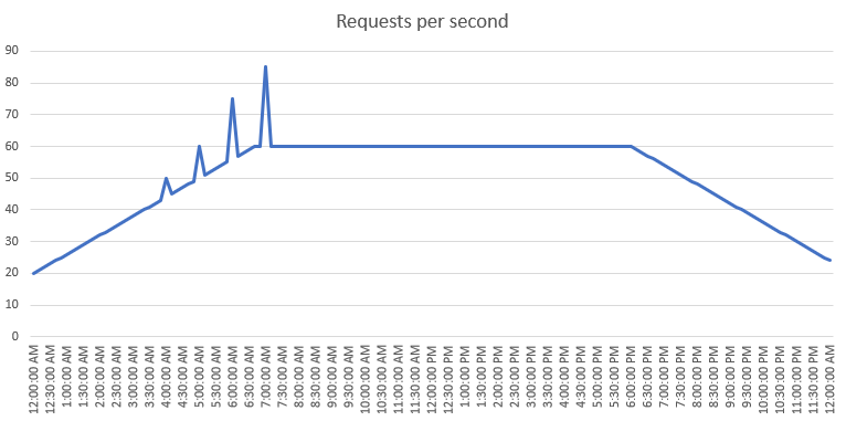
With this information in hands, you can start modelling the observed curve to a discrete table by separating the general smooth load increases and decreases from the spikes (see the snippet below the table). Later on, this table will facilitate configuring Gatling through its API functions.
| Time | Load |
|---|---|
| 00:00 - 07:00 | 20 req/sec - 60 req/sec |
| 07:00 - 18:00 | 60 req/sec - 60 req/sec |
| 18:00 - 00:00 | 60 req/sec - 20 req/sec |
| 04:00 - 04:05 | Spike +5 req/sec |
| 05:00 - 05:05 | Spike +10 req/sec |
| 06:00 - 06:05 | Spike +20 req/sec |
| 07:00 - 07:05 | Spike +25 req/sec |
The following code shows how you can convert the table above to a Gatling simulation.
val getSmooth =
    scenario("Get Smooth")
      .exec(getRequestHttp)

val getPeaks =
    scenario("Get Peaks")
      .exec(getRequestHttp)

setUp(
    // Smooth load curve
    getSmooth.inject(
      // 00:00 -> 07:00
      rampUsersPerSec(scaleLoad(20)).to(scaleLoad(60)).during(scaleTime(7.hours)),
      // 07:00 -> 18:00
      constantUsersPerSec(scaleLoad(60)).during(scaleTime(11.hours)),
      // 18:00 -> 00:00
      rampUsersPerSec(scaleLoad(60)).to(scaleLoad(20)).during(scaleTime(6.hours))
    ),
    // Peaks
    getPeaks.inject(
      // 00:00 -> 04:00
      nothingFor(scaleTime(4.hours)),
      // 04:00 -> 04:05
      constantUsersPerSec(scaleLoad(5)).during(scaleTime(5.minutes)),
      // 04:05 -> 05:00
      nothingFor(scaleTime(55.minutes)),
      // 05:00 -> 05:05
      constantUsersPerSec(scaleLoad(10)).during(scaleTime(5.minutes)),
      // 05:05 -> 06:00
      nothingFor(scaleTime(55.minutes)),
      // 06:00 -> 06:05
      constantUsersPerSec(scaleLoad(20)).during(scaleTime(5.minutes)),
      // 06:05 -> 07:00
      nothingFor(scaleTime(55.minutes)),
      // 07:00 -> 07:05
      constantUsersPerSec(scaleLoad(25)).during(scaleTime(5.minutes))
    )
)
.protocols(httpProtocol)
// We don't assert tests to prevent the pipeline from failing and not extracting the reports
To create a representative set of requests that will be used to emulate your load curve when under tests, you can define a feeder file with various different combinations of parameters and pass it before the exec method. This strategy forces requests to pass randomly through various parts of the source code, avoiding the service from optimizing for a single shape of request. Sometimes you can extract these different combinations by sampling requests from Kibana logs.
val feederGetRequest = csv("request_variations.csv").random

val getRequestHttp = feed(feederGetRequest)
    .exec(
      http("Get Request")
        .get("/endpoint")
        .queryParamMap(Map(
          "query1" -> "#{val1}",
          "query2" -> "#{val2}"
        ))
        .headers(Map(
          "header1" -> "#{val3}",
          "header2" -> "#{val4}"
        ))
        .check(status.in(200, 422))
    )
A drawback of the current Gatling feeder solution is that you can’t have optional parameters in a feeder. For example, if you want header2 to be optional by setting empty values in the CSV file and not sending it as part of the request, it’s not possible. It means that your service has to be able to ignore empty headers. Otherwise, it’ll incur extra complexity for designing your test cases (see SO question).
As you might have noticed, the above code used two functions scaleLoad and scaleTime when setting up the simulation. These functions work in pair with the below properties:
val durationMinutes = System.getProperty("durationMinutes", "60")
val loadFactor = System.getProperty("loadFactor", "1")
These properties enable you to run tests in different setups. For example, you can run the same load scenario for 1 hour or 24 hours by passing those values in minutes through parameters like: --define durationMinutes=60. You can vary the test load by multiplying the scenario configuration by a factor. For example, to run the same scenario with twice the load, you have to set the parameter --define loadFactor=2.0 when running the program. The source code in Gatling used to scale these values is provided below:
def scaleTime(time: FiniteDuration): FiniteDuration = {
  val daySeconds: Double = 86400.0
  val durationSeconds: Double = new FiniteDuration(durationMinutes.toLong, TimeUnit.MINUTES).toSeconds.toDouble
  val unscaledTimeSeconds: Double = time.toSeconds.toDouble
  val scaledTimeSeconds: Double = (durationSeconds / daySeconds) * unscaledTimeSeconds
  val newTime = new FiniteDuration(scaledTimeSeconds.toLong, TimeUnit.SECONDS)
  newTime
}

def scaleLoad(load: Int): Int = {
  val factor: Double = loadFactor.toDouble
  val newLoad = (load * factor).ceil.toInt
  newLoad
}
Setting up execution on Jenkins
When you are done developing the Gatling simulation, the next step is to find a way to run these tests every time you need to do so. For this task, both Jenkins and Kubernetes can be selected as the main tools. The main reason for such a selection is that they allow you to standardize the test platform and minimize potential differences that could appear when running the tests from different developer machines and networks, consequently giving you more consistent results across many runs.
A general pipeline plan to run the tests is given below:
- The pipeline starts by asking for inputs regarding:
- The Gatling class to run the simulation;
- The duration time in minutes;
- The load factor;
- The endpoint URL to run the tests against.
- Next, it starts the execution by:
- Creating a Gatling Agent POD on Kubernetes to run the tests;
- Downloading the repository from Git with the test code;
- Starting the test execution passing the parameters input.
- When the test execution finishes, the pipeline wraps up by:
- Skipping any failure signal so as not to prevent storing the results;
- Uploading the test results as a zip file into an S3 bucket.
As a quick note, be aware that running this kind of performance test on Jenkins will require you not to shut down the job before the end of the execution. The reasoning is that for some situations you might want to simulate a whole day of operation (24 hours).
A not mentioned advantage of this strategy is that when your target workload runs in the cloud, and you run the test agent in the same Cloud region (if possible, the same data center), this will give you lower latency variation when making HTTP calls, and hence more consistent results across many runs.
For this strategy, a pending improvement is that for certain high load factors, the single POD agent running the test saturates with too many requests per second (I have observed that when reaching 800 req/sec). Therefore, one idea for the future could be to spread the load across more Gatling PODs.
Conducting Performance Test Experiments
When running performance tests, a common goal usually is to fine-tune the application so it can handle more load of requests in a resilient and performant way. Starting from the principle you have modelled your application load curve as described previously and automatized it using Jenkins, you are already in a good position to model an experiment and start fine tuning your application.
Assuming you know what critical parameters you want to optimize for your application (a.k.a.: experiment input), you should start with a baseline run and from there change specific parameters to see which one causes the most impact on your application performance. To allow you to measure your application resilience and performance, you also need to define which metrics you are going to use to define the success of your optimizations (a.k.a.: experiment output). In this sense, you can measure whatever metrics you consider being part of a successful application in your context. It’s important to note that when running an experiment all output values are measured from within the time duration the performance test took place.
For illustrating how this experiment would work, the following example depicts a fictional scenario aiming to optimize a standard micro-service communicating to an Auroral SQL DB.
| Type | Variable | Description | Base value |
|---|---|---|---|
| Input | CPU | CPU allocated to POD | req/lim: 500mi |
| Input | Memory | Memory allocated to POD | req/lim: 1Gi |
| Input | DB Connection | Size o DB connection pool | 300 |
| Input | CPU Target | HPA Tracked CPU target for auto-scaling | 75% |
| Input | Database size | Size of the Aurora Database | db.r5.large |
| Input | Min PODs | Minimun number of active PODs | 4 |
| Output | Error Rate | Count of 5XX request responses | - |
| Output | 99th response time | 99th percentile time to respond a request | - |
| Output | Num maximum of PODs | Count peak of running PODs | - |
| Output | Max DB connections | Maximum number of DB connections open | - |
| Outout | Max DB CPU | Maximum DB CPU usage | - |
When running experiment simmulations, it is very important to isolate the test environment so that no external actions take place in parallel with the running tests. Otherwise, this could generate a lot of noise on the collected metrics. Another important aspect is to repeat the same experiment a few times when the probject allows time to do so. In most cases there is not enough time to run enough tests to do confidence analysis using statistical methods. However, make your best to run each experiment at least two or three times.
When you run the first baseline experiment to get the base outputs (see the table below), then you can start variating one variable each time to evaluate which contributes the most to improving the system resilience and performance. The table below depicts a fictional scenario where each param was varied and experimented once to assess its impact on the system.
| Scenario | Erro Rate | 99th response time | Num maximum of PODs | Max DB Connections | Max DB CPU |
|---|---|---|---|---|---|
| Baseline | 1% | 3232 | 3 | 589 | 50% |
| CPU, req/lim: 2000mi | 0.3% | 1232 | 2 | 489 | 45% |
| Memory, req/lim: 4Gi | 1% | 3122 | 3 | 570 | 50% |
| DB Connections, 400 | 0.8% | 2232 | 3 | 789 | 60% |
| CPU Target, 50% | 0.7% | 2232 | 1 | 719 | 55% |
| Database size, db.r5.xlarge | 0.8% | 2232 | 2 | 652 | 20% |
| Min PODs | 0.9% | 2351 | 3 | 517 | 60% |
By analyzing the table above, if we had to select the two best optimization params, a reasonable choice would be the CPU and CPU Target as they reduced the most the error rate (considering this was the main optimizing goal). On the other side, if we were focusing on optimizing the load on the database side, maybe the best options could be the combination of CPU and Database size. The point is, considering the analysis you are conducting, this table is very helpful because it allows you to trade-off what are the most important decisions you could take considering the current context you are in.
Because this is an iterative process, after you apply the fine-tuning from your experiment’s final analysis, you can repeat the same process and keep going this way until you get to a point where the team/company feels comfortable with the decisions made.
Conclusions
Critical systems made for scalability in a resilient and performant way are made on top of experimental methods. Like in science we hypothesize, experiment, and draw conclusions, and keep doing this way until we reach a point where the team feels comfortable to release a new version of the system to the wide public.
Every system has its peculiarities, and an architecture that worked for one project doesn’t guarantee it will work for another project. It means that creating tailored experiments for each project brings lots of value, as you can customize the requests and metrics that are more important for that system analysis.
Before taking this route, also consider how important it’s for your project to reach a certain level of resilience and scalability. Some systems are more critical than others and require more rigor in the decisions made, which means, in many cases very simple systems might not go under this experimental path as it can be expensive to conduct for the company.